아ㅏㅏㅏㅏㅏㅏ 농띠 치고싶은데
너무 놀았다
지금까지 사용한 칼만필터는
시스템 모델이 선형 모델인 경우에만 사용 가능하였다.
하지만 실제 현실 현상은 비선형 모델인 경우가 많은데
이를 칼만 필터로 모델링하기 위해
1차 태일러 전개로 비선형 모델을 선형화해서 사용하게 되었음
뭐가 비선형 시스템인지 아닌지는
이전에 파이썬 로보틱스인가 다른데서 메트랩 코드 보고 이해했었는지 가물가물한데
EKF 로봇 위치 추정 따라 구현하면서 꽤 이해됬었지만
설명하라면 잘 못하겠다.
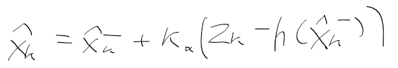
일단 기존에 칼만 필터는 행렬을 사용했지만 비선형 시스템 모델을 다루기 위해선 비선형 함수를 사용함

비선형 함수로 바뀌면서 X 추정치도 이런식으로 바뀐다
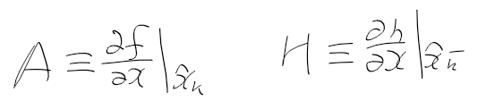
그러면 기존의 A, H 자리에 들어가는건 비선형 함수 f, h를 x로 편미분 시켜준게 들어간다.
뭔 소린가 싶겠지만 코드 보는게 나을듯
1. EKF를 이용한 레이더 추적
조건 : 물체는 고도, 속도 일정함
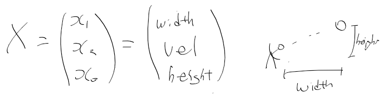
상태 : 수평 거리, 속도, 고도
모르는거 : 속도, 고도
* 수평 거리와 고도를 자주 쓰는 단어인 width, height로 대충 적음
horizontal distance나 vertical distance 쓰자니 안맞는것 같기도하고 너무 길어
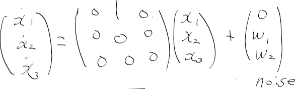
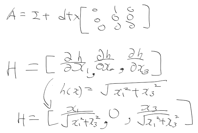
고도, 속도가 일정하다는 조건을 따르면
A행렬은 이런식이되고, 속도가 일정 = 노이즈가 없다(?)라 치면 시스템 모델은 이런식으로 정리된다.
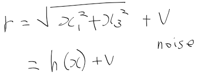
측정 모델같은 경우
레이더서 물체까지 직선 거리, 유클리디안 거리를 얻는데 이 거리는
sqrt(width **2 + height **2)로부터 얻을수 있으므로 노이즈 포함하면 이런식이됨
대충 관측치를 갖고 width, vel, height 다 계산해내갯다는거같은데
그러면 수평 거리만 알고 속도, 고도는 모른다는건 왜 그런걸까?
수평 거리, 속도, 고도 다 모른다해도 되지않나
일단 지금 작성한 모델들을 보면
시스템 모델은 선형 시스템이나, 관측 모델은 비선형이므로 선형화 해야함
선형화라 해봤자 우리가 자주 아는 편미분해서 편도함수 (자코비안)구하면됨
문제 ! 처음 시작할때 초기값 X가 없다.
X가 없으면 EKF(자코비안) 계산할수 없기도하고,
잘못된거 넣으면 오차가 발산하게되므로
초기 상태에 가장 잘 맞는 초기 추정치 X를 잘 설정해줘야 함
대충 ekf 구현 결과
import numpy as np
from math import sqrt

def jacobian(X_est):
    H = np.array([[0, 0, 0]])
    x1 = X_est[0][0]
    x3 = X_est[2][0]
    H[0][0] = x1 / sqrt(x1 ** 2 + x3 ** 2)
    H[0][2] = x3 / sqrt(x1 ** 2 + x3 ** 2)
    return H

def hx(X_pred):
    x1 = X_pred[0][0] # width
    x3 = X_pred[2][0] # height
    z_pred = sqrt(x1 ** 2 + x3 **2)
    return z_pred

dt = 0.05

A = np.array([
    [0, 1, 0],
    [0, 0, 0],
    [0, 0, 0]
])
A = np.eye(3) + dt * A
Q = np.array([
    [0, 0, 0],
    [0, 0.001, 0],
    [0, 0, 0.001]
])
R = 10
X = np.array([
    [0, 90, 1100]
]).T
P = 10 * np.eye(3)

H = jacobian(X)

def ekf(z):
    X_pred = A @ X
    P_pred = A @ P @ A.T + Q
    K = P_pred @ H.T @ np.linalg.inv(H @ P_pred @ H.T + R)
    X_est = X_pred + K @ (z - hx(X_pred))
    P_est = P_pred - K @ H @ P_pred
    return X_est, P_est
이걸 실제 동작 코드랑 합쳐줘야 한다
그전에 레이더 데이터 로드부터 구현하면..
아 고도 altitude가 있었네
그래도 그냥 매트랩 따라적음
고도는 1000으로 고정하고 노이즈 추가
속도도 100으로 고정하고 노이즈 추가
고도, 수평 거리로 직선 거리 계산하고 노이즈 추가 후 반환
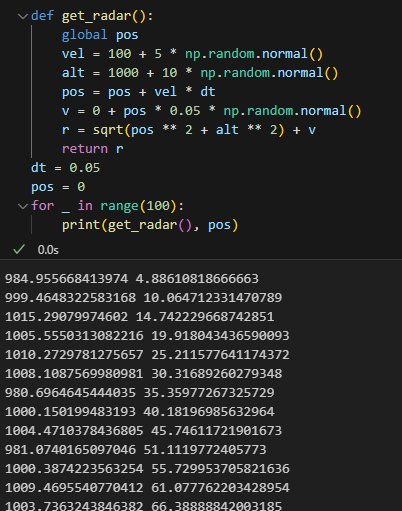
def get_radar():
    global pos
    vel = 100 + 5 * np.random.normal()
    alt = 1000 + 10 * np.random.normal()
    pos = pos + vel * dt
    v = 0 + pos * 0.05 * np.random.normal()
    r = sqrt(pos ** 2 + alt ** 2) + v
    return r
dt = 0.05
pos = 0
for _ in range(100):
    print(get_radar(), pos)
레이더 데이터 가져오기도 구현했으니
아까 구현한 EKF랑 데이터 플로팅을 합치면된다.
하고 구현하고보니
중간에 잘못 만든게 몇개 있어서 한참 찾아해맴
자코비안 계산중에 dtype을 float32안해줬더니
자동으로 int로 설정되서 그런가
자코비안 행렬 H가 자꾸 값이 0으로만 나오는것떄문에 --
아무튼 계산 결과도 잘 나온다
위치는 0 에서 계속 100씩 올라가가고
속도는 실제는 100인데, 초기치로 90을 줘서 잠깐 요동치다 대충 맞추고
고도 같은 경우 실제 1000이지만 초기치를 1100으로 줘서 처음엔 위에서 급떨어진다
직선 거리같은 경우에는 잘 필터링해서 따라간다.

import numpy as np
import matplotlib.pyplot as plt
from math import sqrt

def jacobian(X_est):
    H = np.array([[0, 0, 0]], dtype=np.float32)
    x1 = X_est[0][0]
    x3 = X_est[2][0]
    H[0][0] = x1 / sqrt(x1 ** 2 + x3 ** 2)
    H[0][2] = x3 / sqrt(x1 ** 2 + x3 ** 2)
    return H

def hx(X_pred):
    x1 = X_pred[0][0] # width
    x3 = X_pred[2][0] # height
    z_pred = sqrt(x1 ** 2 + x3 **2)
    return z_pred

def get_radar():
    global pos
    vel = 100 + 5 * np.random.normal()
    alt = 1000 + 10 * np.random.normal()
    pos = pos + vel * dt
    v = 0 + pos * 0.05 * np.random.normal()
    r = sqrt(pos ** 2 + alt ** 2) + v
    return r

def ekf(X, P, z):
    X_pred = A @ X
    P_pred = A @ P @ A.T + Q
    K = P_pred @ H.T @ np.linalg.inv(H @ P_pred @ H.T + R)
    X_est = X_pred + K * (z - hx(X_pred))
    P_est = P_pred - K @ H @ P_pred
    return X_est, P_est

dt = 0.05
pos = 0
t_list = np.arange(0, 20, 0.05)
pos_list, vel_list, alt_list, z_list, dist_list = [], [], [], [], []

A = np.array([
    [0, 1, 0],
    [0, 0, 0],
    [0, 0, 0]
])
A = np.eye(3) + dt * A
Q = np.array([
    [0, 0, 0],
    [0, 0.001, 0],
    [0, 0, 0.001]
])
R = 10
X_est = np.array([
    [0, 90, 1100]
]).T
P_est = 10 * np.eye(3)

for _ in range(len(t_list)):
    H = jacobian(X_est)
    z = get_radar()
    X_est, P_est = ekf(X_est, P_est, z)
    pos_list.append(X_est[0][0])
    vel_list.append(X_est[1][0])
    alt_list.append(X_est[2][0])
    z_list.append(z)
    dist_list.append(sqrt(X_est[0][0] ** 2 + X_est[2][0] ** 2))

plt.subplot(411)
ax1 = plt.subplot(4,1,1)
ax2 = plt.subplot(4,1,2)
ax3 = plt.subplot(4,1,3)
ax4 = plt.subplot(4,1,4)
ax1.plot(t_list, pos_list, label="pos")
ax2.plot(t_list, vel_list, label="vel")
ax3.plot(t_list, alt_list, label="alt")
ax4.plot(t_list, z_list, label="measured")
ax4.plot(t_list, dist_list, label="estimated")
ax1.legend()
ax2.legend()
ax3.legend()
ax4.legend()
2. 오일러각 EKF 적용하기
지난 글에 작성한 자이로, 가속도계 데이터에 칼만필터를 사용했는데
이번에는 오일러각을 EKF로 구해보려고한다.
칼만 필터로 오일러각 계산할때는 각속도 p,q,r로 행렬 A를 놓고 phi, theta, psi를 계산할수 없어서
쿼터니언으로 변환해서 사용했었다.
그때 사용한 행렬 A는 다음 같은 식인데
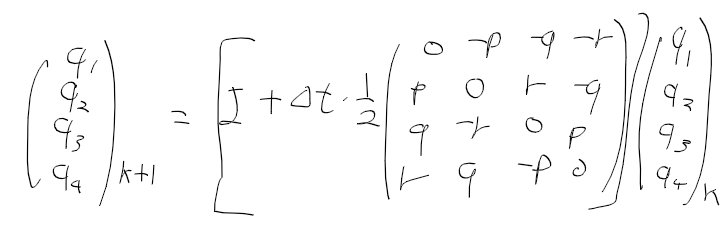
EKF로 비선형 함수를 선형화해서 쓰면 p, q, r로도 phi, theta, psi를 계산할수 있다
일단 p, q, r과 파이 세타 프사이 관계는 이런식
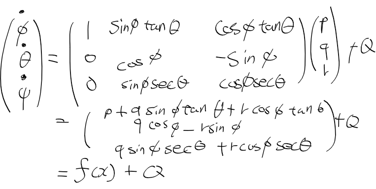
하지만 EKF에선 비선형 함수를 선형화해서 자코비안 행렬로 시스템 모델 A를 구할수 있음

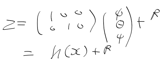
관측 모델의 경우 가속도계로 파이, 세타만 구하였으므로
H는 다음 형태가 된다.
이제 대충 내용 정리됬으니 기존 자이로, 가속도 센서 퓨전 코드를 EKF로 고쳐보면
기본 로직은 이런식으로
dt = 0.01
t_list = np.linspace(0, 415, 41500)
phi_list, theta_list, psi_list = [], [], []

X_est = np.array([[0, 0, 0]]).T
P_est = 10 * np.eye(3)

H = np.array([
    [1, 0, 0],
    [0, 1, 0]
])
Q = np.array([
    [0.0001, 0, 0],
    [0, 0.0001, 0],
    [0, 0, 0.1]
])
R = 10 * np.eye(2)

for (p, q, r), (ax, ay, az) in zip(get_gyro(), get_accel()):

    rates = (p, q, r)
    phi, theta = accel_euler(ax, ay, az)
    z = np.array([[phi, theta]]).T
    X_est, P_est = ekf_euler(z, rates, X_est, P_est, dt)

    phi_list.append(X_est[0][0] * 180 / pi)
    theta_list.append(X_est[1][0] * 180 / pi)
    psi_list.append(X_est[2][0] * 180 / pi)


plt.subplot(311)
ax1 = plt.subplot(3,1,1)
ax2 = plt.subplot(3,1,2)
ax3 = plt.subplot(3,1,3)
ax1.plot(t_list, phi_list)
ax2.plot(t_list, theta_list)
ax3.plot(t_list, psi_list)
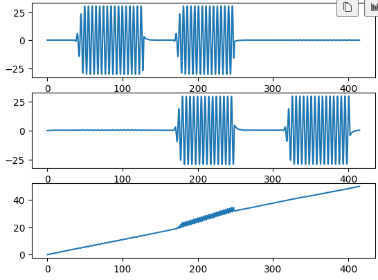
오일러각 ekf에서
이전 X_est와 가져온 p, q, r rates로 비선형 함수 fx와 자코비안 A 계산
이후 X_est와 P_est 계산해서 반환하면 파이와 세타는 지난글 오일러각 구한것과 비슷하게 나오는데
프사이는 좀 다르다 뭘 틀리게 한건질 모르겟네
def fx(X_est, rates, dt):
    phi = X_est[0][0]
    theta = X_est[1][0]

    p = rates[0]
    q = rates[1]
    r = rates[2]

    X_pred = np.array([[0, 0, 0]], dtype=np.float32).T
    X_pred[0][0] = p + q * sin(phi) * tan(theta) + r * cos(phi) * tan(theta)
    X_pred[1][0] = q * cos(phi) - r * sin(phi)
    X_pred[2][0] = q * sin(phi) / cos(theta) + r * cos(phi) / cos(theta)
    # math에는 sec가 없어서 sec는 cos의 역수이므로 곱 sec 대신 / cos로 계산

    X_pred = X_est + X_pred * dt
    return X_pred


def jacob_A(X_est, rates, dt):
    phi = X_est[0][0]
    theta = X_est[1][0]

    p = rates[0]
    q = rates[1]
    r = rates[2]

    A = np.zeros((3, 3), dtype=np.float32)
    A[0, 0] = q * cos(phi) * tan(theta) - r * sin(phi) * tan(theta)
    A[0, 1] = q * sin(phi) / (cos(theta)**2) + r * cos(phi) / (cos(theta)**2)
    A[0, 2] = 0

    A[1, 0] = -q * sin(phi) - r * cos(phi)
    A[1, 1] = 0
    A[1, 2] = 0

    A[2, 0] = q * cos(phi) / cos(theta) - r * sin(phi) / cos(theta)
    A[2, 1] = q * sin(phi) / cos(theta) * tan(theta) + r * cos(phi) / cos(theta) * tan(theta)
    A[2, 2] = 0

    A = np.eye(3) + A * dt
    return A


def accel_euler(ax, ay, az):
    g = 9.8
    theta = asin( ax / g)
    phi = asin(-ay / (g * cos(theta)))
    return phi, theta


def ekf_euler(z, rates, X_est, P_est, dt):
    A = jacob_A(X_est, rates, dt)
    X_pred = fx(X_est, rates, dt)
    P_pred = A @ P_est @ A.T + Q
    K = P_pred @ H.T @ np.linalg.inv(H @ P_pred @ H.T + R)
    X_est = X_pred + K @ (z - H @ X_pred)
    P_est = P_pred - K @ H @ P_pred
    return X_est, P_est
자이로, 가속도계 EKF를 이용한 센서 퓨전 전체 코드
from math import atan2, sin, cos, asin, tan
from math import pi
import scipy.io
import matplotlib.pyplot as plt
import numpy as np

gyro = scipy.io.loadmat("EulerEKF/ArsGyro.mat")
def get_gyro():
    wx = gyro["wx"]
    wy = gyro["wy"]
    wz = gyro["wz"]

    gyro_len = len(wx)
    for i in range(gyro_len):
        yield wx[i][0], wy[i][0], wz[i][0]

accel = scipy.io.loadmat("EulerEKF/ArsAccel.mat")
def get_accel():
    ax = accel["fx"]
    ay = accel["fy"]
    az = accel["fz"]

    accel_len = len(ax)
    for i in range(accel_len):
        yield ax[i][0], ay[i][0], az[i][0]


def fx(X_est, rates, dt):
    phi = X_est[0][0]
    theta = X_est[1][0]

    p = rates[0]
    q = rates[1]
    r = rates[2]

    X_pred = np.array([[0, 0, 0]], dtype=np.float32).T
    X_pred[0][0] = p + q * sin(phi) * tan(theta) + r * cos(phi) * tan(theta)
    X_pred[1][0] = q * cos(phi) - r * sin(phi)
    X_pred[2][0] = q * sin(phi) / cos(theta) + r * cos(phi) / cos(theta)
    # math에는 sec가 없어서 sec는 cos의 역수이므로 곱 sec 대신 / cos로 계산

    X_pred = X_est + X_pred * dt
    return X_pred


def jacob_A(X_est, rates, dt):
    phi = X_est[0][0]
    theta = X_est[1][0]

    p = rates[0]
    q = rates[1]
    r = rates[2]

    A = np.zeros((3, 3), dtype=np.float32)
    A[0, 0] = q * cos(phi) * tan(theta) - r * sin(phi) * tan(theta)
    A[0, 1] = q * sin(phi) / (cos(theta)**2) + r * cos(phi) / (cos(theta)**2)
    A[0, 2] = 0

    A[1, 0] = -q * sin(phi) - r * cos(phi)
    A[1, 1] = 0
    A[1, 2] = 0

    A[2, 0] = q * cos(phi) / cos(theta) - r * sin(phi) / cos(theta)
    A[2, 1] = q * sin(phi) / cos(theta) * tan(theta) + r * cos(phi) / cos(theta) * tan(theta)
    A[2, 2] = 0

    A = np.eye(3) + A * dt
    return A


def accel_euler(ax, ay, az):
    g = 9.8
    theta = asin( ax / g)
    phi = asin(-ay / (g * cos(theta)))
    return phi, theta


def ekf_euler(z, rates, X_est, P_est, dt):
    A = jacob_A(X_est, rates, dt)
    X_pred = fx(X_est, rates, dt)
    P_pred = A @ P_est @ A.T + Q
    K = P_pred @ H.T @ np.linalg.inv(H @ P_pred @ H.T + R)
    X_est = X_pred + K @ (z - H @ X_pred)
    P_est = P_pred - K @ H @ P_pred
    return X_est, P_est

dt = 0.01
t_list = np.linspace(0, 415, 41500)
phi_list, theta_list, psi_list = [], [], []

X_est = np.array([[0, 0, 0]]).T
P_est = 10 * np.eye(3)

H = np.array([
    [1, 0, 0],
    [0, 1, 0]
])
Q = np.array([
    [0.0001, 0, 0],
    [0, 0.0001, 0],
    [0, 0, 0.1]
])
R = 10 * np.eye(2)

for (p, q, r), (ax, ay, az) in zip(get_gyro(), get_accel()):

    rates = (p, q, r)
    phi, theta = accel_euler(ax, ay, az)
    z = np.array([[phi, theta]]).T
    X_est, P_est = ekf_euler(z, rates, X_est, P_est, dt)

    phi_list.append(X_est[0][0] * 180 / pi)
    theta_list.append(X_est[1][0] * 180 / pi)
    psi_list.append(X_est[2][0] * 180 / pi)


plt.subplot(311)
ax1 = plt.subplot(3,1,1)
ax2 = plt.subplot(3,1,2)
ax3 = plt.subplot(3,1,3)
ax1.plot(t_list, phi_list)
ax2.plot(t_list, theta_list)
ax3.plot(t_list, psi_list)
'컴퓨터과학 > 필터' 카테고리의 다른 글
| 칼만필터 파이썬 - 10. 파티클 필터 구현하기(실패) (0) | 2023.10.05 |
|---|---|
| 칼만필터 파이썬 - 9. 무향 칼만 필터 (0) | 2023.10.04 |
| 칼만필터 파이썬 - 7. 칼만필터를 이용한 가속도계와 자이로 센서 퓨전 (0) | 2023.10.04 |
| 칼만필터 파이썬 - 6. 칼만 필터를 이용한 추적기 구현 (0) | 2023.10.03 |
| 칼만필터 파이썬 - 5. 칼만 필터를 이용한 위치로 속도 계산 (0) | 2023.10.02 |