이전까지는 각 관절들의 RPY를 계산해서 제어하겠다고 해매고 다녔는데
RPY 다루기전에 location 을 이용하면 쉽게 만들수 있는건 알고 있었다.
그럼에도 나중에 만들걸 생각하면 RPY를 이해해야해서 해멘건데
일단 대충 이해했으니 이젠 좌표기반으로 손관절을 이동시켜보려고한다.
이전에는 본 로테이션만 다뤘는데
로케이션도 컴포넌트 공간에서 좌표이동이 가능

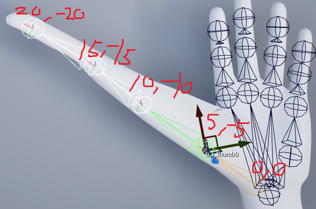
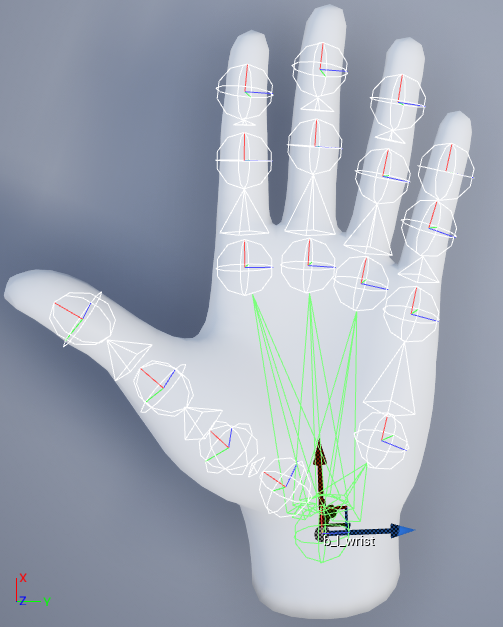
컴포넌트 좌표계와 위치를 보면 이런식으로 됨

x 20줄때

y -20 준결과
그런데 생각한거랑 좀 다른게
thumb2에 xy 15, -15를 줫더니
썸3이 더멀어졌다 내가 원한건 아닌데

다시 해서
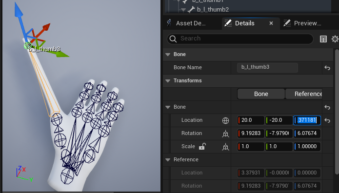
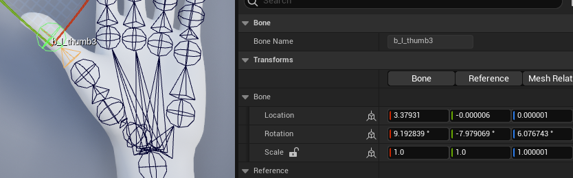
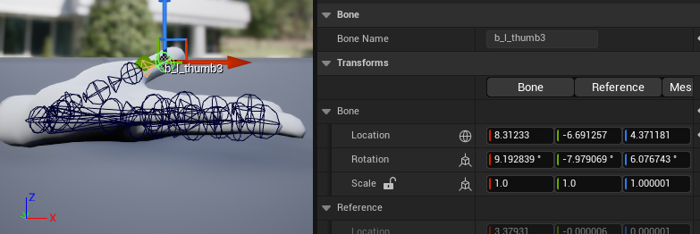
썸 2에 15, -15주고
썸3을봄녀 전역계 17.3, -17.2 정도 나온다.

이때 썸3의 로컬계는 3.3, 0 정돈데

초기 로컬계 값이 그대로 유지되기때문으로 생각됨
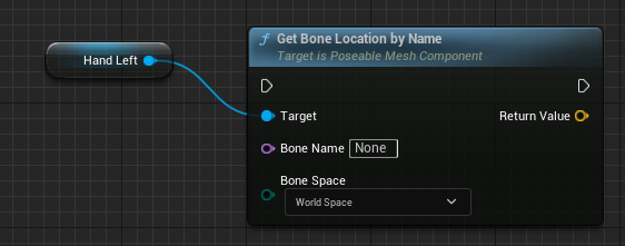
나중에 관절 지나는 선 법선으로 마우스 제어하려고
본 위치도 볼수있나 확인
본 위치도 전역계와 컴포넌트계 둘다 확인가능
본트랜스폼도 취득가능한데 뭔가 다양하다
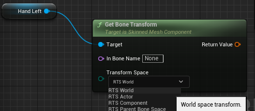
다시 썸으로 돌아와
컴포넌트 계를 부모에서 자식 순서대로 설정하면 원하는 형태로 지정되는듯하다.
컴포넌트 공간으로 엄지, 검지, 중지 위치 설정하는 bp
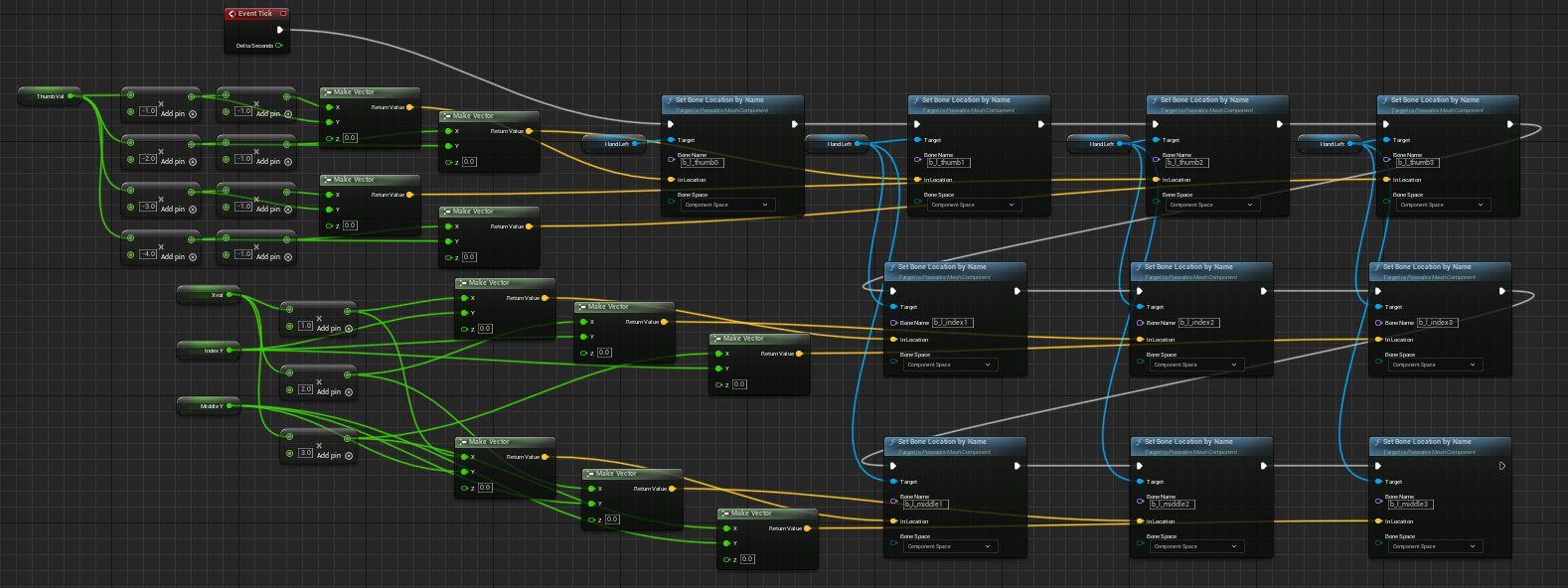
실행결과
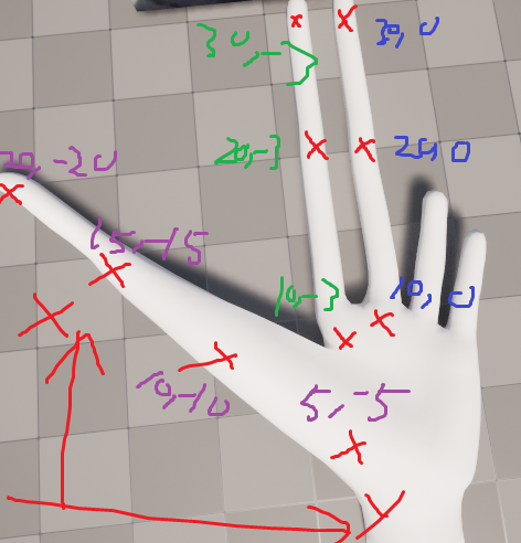
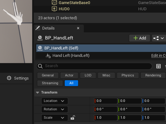
손을 원래 스케일111, rpy는 000로 하고 원점에 놓은상태에서
위 블루프린트 전체 컴포넌트계 대신 전역계바꾸면 아까 한것과 동일하게 나온다.
그러면 블라즈 핸드를 256 x 256으로 반정규화 시켰었는데
이를 스켈레탈메시 기준 컴포넌트 스페이스에서 보려고한다.
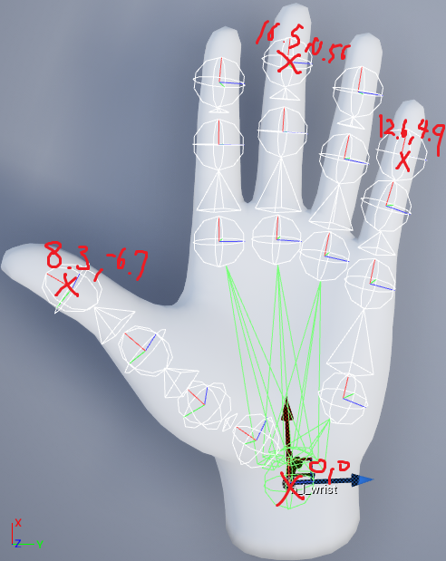
일단 최외각에 있는 4점의 xy좌표만 뽑아오면 이런식이다.
y는 4.9 - (-6.7) = 11.6
x는 16.5 - = 16.5
이므로 x는 16.5, y는 11.6으로 반정규화 하면될듯?
이전에 사용한건 반정규화된 값을 사용했으니
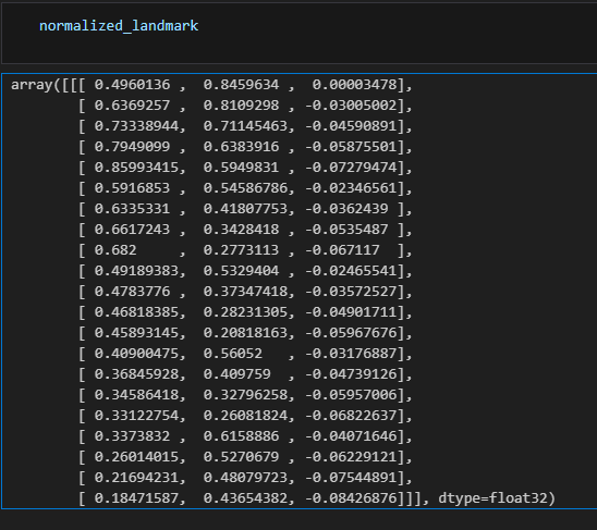
정규화된 랜드마크 값을 보면 이런식으로
xyz 가 모두 0~1사이로 나온다.
x축은 0부터 시작하므로 -0.5 하지않고 그냥 16.5를 곱
y축은 -부터 하므로
y축만 -0.5 한후 11.6을 곱
하면 되지 않을까 싶었는데
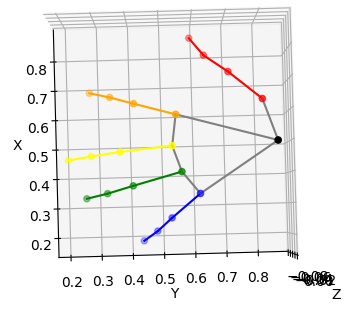
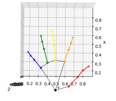
반정규화 된 랜드마크들을 갖고
x가 위를 향하는 xy평면으로 보면
손등을 보고 있는 상태인건 둘째치고 회전된 상태이다.

생각해보니 기존에 저장해둔 넘파이 파일 자채가 정규화된걸 반정규화되서 쓰고있엇네
원래있던거 드로잉하면 이런식
손을 어떻게 회전시켜야되나 고민하다
생각해보니 그냥
xy축 데이터를 바꾸면 끝이엇네?
대신 x가 밑으로 갈수록 커지니
(x - 손목x) * -1을 하면 원래 손 방향대로 갈듯싶은데

import matplotlib.pyplot as plt
import numpy as np
import pandas as pd


%matplotlib widget

# 3차원 산점도 그리기
fig = plt.figure()
ax = fig.add_subplot(111, projection='3d')

x = normalized_landmark[:, 1]
y = normalized_landmark[:, 0]
z = normalized_landmark[:, 2]

# 색상 지정
colors = ['black'] + ['red'] * 4 + ['orange'] * 4 + ['yellow'] * 4 + ['green'] * 4 + ['blue'] * 4
ax.scatter(x, y, z, c=colors)


#손가락
colors = ['red', 'orange', 'yellow', 'green', 'blue']
groups = [[1, 2, 3, 4], [5, 6, 7, 8], [9, 10, 11, 12], [13, 14, 15, 16], [17, 18, 19, 20]]
for i, group in enumerate(groups):
    for j in range(len(group)-1):
        plt.plot([x[group[j]], x[group[j+1]]], [y[group[j]], y[group[j+1]]], [z[group[j]], z[group[j+1]]], color=colors[i])
#손등
lines = [[0, 1], [0, 5], [0, 17], [5, 9], [9, 13], [13, 17]]
for line in lines:
    ax.plot([x[line[0]], x[line[1]]], [y[line[0]], y[line[1]]], [z[line[0]], z[line[1]]], color='gray')


ax.set_xlabel('X')
ax.set_ylabel('Y')
ax.set_zlabel('Z')


plt.gca().invert_xaxis()
plt.show()
xlim이 0.2, 0.8로 설정되었는지 손이 그래프 밖에 나가긴했지만
손목 x를 0으로 보내서 대충 맞춘거같긴한데
y 방향도 맞추고
위에서 찾은 값으로 반정규화도 해주자
import matplotlib.pyplot as plt
import numpy as np
import pandas as pd


%matplotlib widget

# 3차원 산점도 그리기
fig = plt.figure()
ax = fig.add_subplot(111, projection='3d')

x = (normalized_landmark[:, 1] - normalized_landmark[0, 1]) * -1
y = normalized_landmark[:, 0]
z = normalized_landmark[:, 2]

# 색상 지정
colors = ['black'] + ['red'] * 4 + ['orange'] * 4 + ['yellow'] * 4 + ['green'] * 4 + ['blue'] * 4
ax.scatter(x, y, z, c=colors)


#손가락
colors = ['red', 'orange', 'yellow', 'green', 'blue']
groups = [[1, 2, 3, 4], [5, 6, 7, 8], [9, 10, 11, 12], [13, 14, 15, 16], [17, 18, 19, 20]]
for i, group in enumerate(groups):
    for j in range(len(group)-1):
        plt.plot([x[group[j]], x[group[j+1]]], [y[group[j]], y[group[j+1]]], [z[group[j]], z[group[j+1]]], color=colors[i])
#손등
lines = [[0, 1], [0, 5], [0, 17], [5, 9], [9, 13], [13, 17]]
for line in lines:
    ax.plot([x[line[0]], x[line[1]]], [y[line[0]], y[line[1]]], [z[line[0]], z[line[1]]], color='gray')


ax.set_xlabel('X')
ax.set_ylabel('Y')
ax.set_zlabel('Z')
ax.invert_yaxis()

plt.show()
""
x축은 0부터 시작하므로 -0.5 하지않고 그냥 16.5를 곱
y축은 -부터 하므로
y축만 -0.5 한후 11.6을 곱
"""
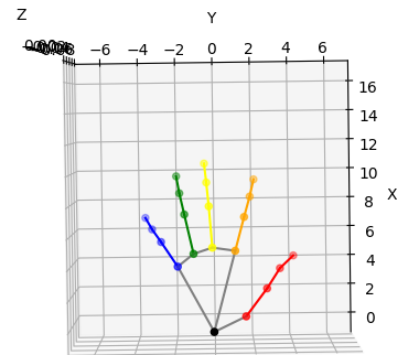
하면 반정규화 랜드마크 가장 큰 x가 10쯤되서 우측그림이랑 잘 안맞긴한데
대충 넘어가고
새끼손가락 끝은 우측그림이 4.9인데 반정규화 결과는 3.9쯤 나오네
반대로 새끼손까락끝은 우측그림 -6.7이나 반정규화 결과는 4.1쯤 나온다 대충 방향이 반대니
y축 데이터에 -를 곱해줘야할듯
 |
|
import matplotlib.pyplot as plt
import numpy as np
import pandas as pd


%matplotlib widget

# 3차원 산점도 그리기
fig = plt.figure()
ax = fig.add_subplot(111, projection='3d')

denormalized_landmark = normalized_landmark.copy()
denormalized_landmark[:,0] = 16.5 * (normalized_landmark[:, 1] - normalized_landmark[0, 1]) * -1
denormalized_landmark[:,1] = (normalized_landmark[:, 0] - 0.5) * 11.6
denormalized_landmark[:,2] = normalized_landmark[:, 2]

x = denormalized_landmark[:, 0]
y = denormalized_landmark[:, 1]
z = denormalized_landmark[:, 2]

# 색상 지정
colors = ['black'] + ['red'] * 4 + ['orange'] * 4 + ['yellow'] * 4 + ['green'] * 4 + ['blue'] * 4
ax.scatter(x, y, z, c=colors)


#손가락
colors = ['red', 'orange', 'yellow', 'green', 'blue']
groups = [[1, 2, 3, 4], [5, 6, 7, 8], [9, 10, 11, 12], [13, 14, 15, 16], [17, 18, 19, 20]]
for i, group in enumerate(groups):
    for j in range(len(group)-1):
        plt.plot([x[group[j]], x[group[j+1]]], [y[group[j]], y[group[j+1]]], [z[group[j]], z[group[j+1]]], color=colors[i])
#손등
lines = [[0, 1], [0, 5], [0, 17], [5, 9], [9, 13], [13, 17]]
for line in lines:
    ax.plot([x[line[0]], x[line[1]]], [y[line[0]], y[line[1]]], [z[line[0]], z[line[1]]], color='gray')


ax.set_xlabel('X')
ax.set_ylabel('Y')
ax.set_zlabel('Z')


ax.set_xlim(-1, 17)
ax.set_ylim(7, -7)


plt.show()
이제 컴포넌트 공간 좌표들과
xy가 얼추 비슷해졌다.
 |
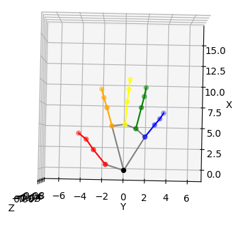 |
| y축 데이터 -1곱전 | -1 곱후 |

import matplotlib.pyplot as plt
import numpy as np
import pandas as pd


%matplotlib widget

# 3차원 산점도 그리기
fig = plt.figure()
ax = fig.add_subplot(111, projection='3d')

denormalized_landmark = normalized_landmark.copy()
denormalized_landmark[:,0] = 16.5 * (normalized_landmark[:, 1] - normalized_landmark[0, 1]) * -1
denormalized_landmark[:,1] = (normalized_landmark[:, 0] - 0.5) * 11.6 * -1
denormalized_landmark[:,2] = normalized_landmark[:, 2]

x = denormalized_landmark[:, 0]
y = denormalized_landmark[:, 1]
z = denormalized_landmark[:, 2]

# 색상 지정
colors = ['black'] + ['red'] * 4 + ['orange'] * 4 + ['yellow'] * 4 + ['green'] * 4 + ['blue'] * 4
ax.scatter(x, y, z, c=colors)


#손가락
colors = ['red', 'orange', 'yellow', 'green', 'blue']
groups = [[1, 2, 3, 4], [5, 6, 7, 8], [9, 10, 11, 12], [13, 14, 15, 16], [17, 18, 19, 20]]
for i, group in enumerate(groups):
    for j in range(len(group)-1):
        plt.plot([x[group[j]], x[group[j+1]]], [y[group[j]], y[group[j+1]]], [z[group[j]], z[group[j+1]]], color=colors[i])
#손등
lines = [[0, 1], [0, 5], [0, 17], [5, 9], [9, 13], [13, 17]]
for line in lines:
    ax.plot([x[line[0]], x[line[1]]], [y[line[0]], y[line[1]]], [z[line[0]], z[line[1]]], color='gray')


ax.set_xlabel('X')
ax.set_ylabel('Y')
ax.set_zlabel('Z')


ax.set_xlim(-1, 17)
ax.set_ylim(7, -7)


plt.show()
마지막으로 z축 데이터도 맞춰줘야하는데
보통 블라즈 핸드 z축 데이터는 height값을 곱해서 반정규화 시켜주므로
11.6을 곱해주려고 하는데
정규화된 z축 데이터는 -방향이 되어있으므로
z축 데이터는 11.6 * -1을 곱해 반정규화를 시켜보려한다.
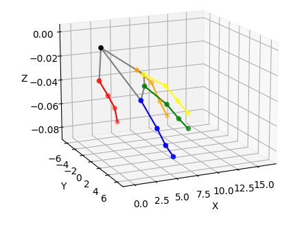
반정규화 결과 z축 값이 손을 원래 편채로 했을때 데이터라 그런지 좀 작은 편이긴하지만
왼손 모델과 동일한 좌표계로 만들었다.
이 데이터를 그대로 컴포넌트 좌표계로 세팅하면 될듯

import matplotlib.pyplot as plt
import numpy as np
import pandas as pd


%matplotlib widget

# 3차원 산점도 그리기
fig = plt.figure()
ax = fig.add_subplot(111, projection='3d')

denormalized_landmark = normalized_landmark.copy()
denormalized_landmark[:,0] = 16.5 * (normalized_landmark[:, 1] - normalized_landmark[0, 1]) * -1
denormalized_landmark[:,1] = (normalized_landmark[:, 0] - 0.5) * 11.6 * -1
denormalized_landmark[:,2] = normalized_landmark[:, 2] * 11.6 * -1

x = denormalized_landmark[:, 0]
y = denormalized_landmark[:, 1]
z = denormalized_landmark[:, 2]

# 색상 지정
colors = ['black'] + ['red'] * 4 + ['orange'] * 4 + ['yellow'] * 4 + ['green'] * 4 + ['blue'] * 4
ax.scatter(x, y, z, c=colors)


#손가락
colors = ['red', 'orange', 'yellow', 'green', 'blue']
groups = [[1, 2, 3, 4], [5, 6, 7, 8], [9, 10, 11, 12], [13, 14, 15, 16], [17, 18, 19, 20]]
for i, group in enumerate(groups):
    for j in range(len(group)-1):
        plt.plot([x[group[j]], x[group[j+1]]], [y[group[j]], y[group[j+1]]], [z[group[j]], z[group[j+1]]], color=colors[i])
#손등
lines = [[0, 1], [0, 5], [0, 17], [5, 9], [9, 13], [13, 17]]
for line in lines:
    ax.plot([x[line[0]], x[line[1]]], [y[line[0]], y[line[1]]], [z[line[0]], z[line[1]]], color='gray')


ax.set_xlabel('X')
ax.set_ylabel('Y')
ax.set_zlabel('Z')


ax.set_xlim(-1, 17)
ax.set_ylim(7, -7)
ax.set_zlim(0, 2)


plt.show()
사용한 정규화된 랜드마크 넘파이 파일
import numpy as np


normalized_landmark = np.load("normalized_landmarks2.npy")
np.set_printoptions(suppress=True)
denormalize_landmark = normalized_landmark.copy()
denormalize_landmark[:,:,2] = normalized_landmark[:,:,2] * (256)
denormalize_landmark[:,:,:2]  = normalized_landmark[:,:,:2] * 256
denormalize_landmark
denormalize_landmark = denormalize_landmark.squeeze()
denormalize_landmark.shape
'컴퓨터과학 > 언리얼' 카테고리의 다른 글
| HandDesktop18 - 카메라 중점, 줌 거리 찾기 (0) | 2024.02.05 |
|---|---|
| HandDesktop17 - 손 관절 가지고 놀기5 좌표로 다루기 구현 (0) | 2024.02.02 |
| HandDesktop15 - 손 관절 가지고 놀기3 손이동 구현 (0) | 2024.02.01 |
| HandDesktop14 - 손 관절 가지고 놀기2 컴포넌트공간 관절회전 (0) | 2024.02.01 |
| HandDesktop13 - 손 관절 가지고 놀기 (0) | 2024.02.01 |