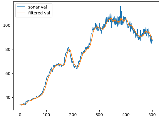
import scipy.io

sonar = scipy.io.loadmat("SonarAlt.mat")

def get_sonar():
    sonar_arr = sonar["sonarAlt"][0]
    sonar_len = len(sonar_arr)
    for i in range(sonar_len):
        yield sonar_arr[i]

for val in get_sonar():
    print(val)
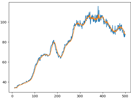
import scipy.io

sonar = scipy.io.loadmat("SonarAlt.mat")

def get_sonar():
    sonar_arr = sonar["sonarAlt"][0]
    sonar_len = len(sonar_arr)
    for i in range(sonar_len):
        yield sonar_arr[i]

for val in get_sonar():
    print(val)
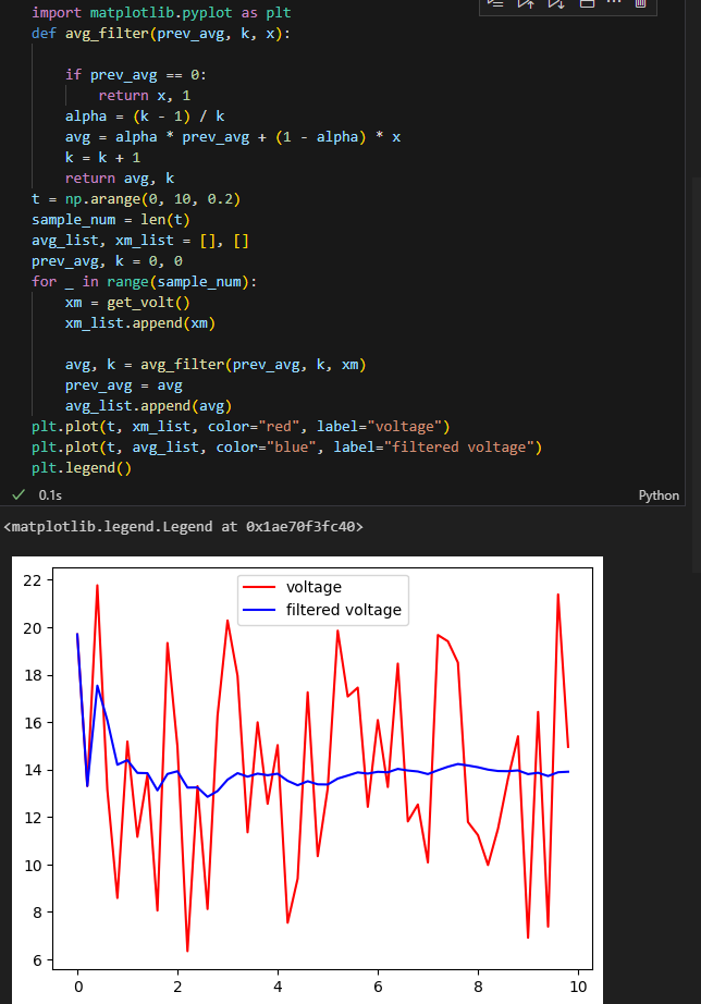
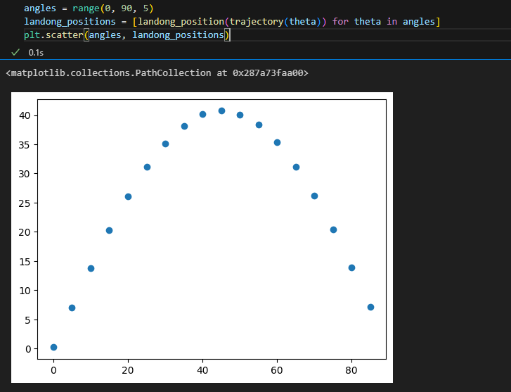
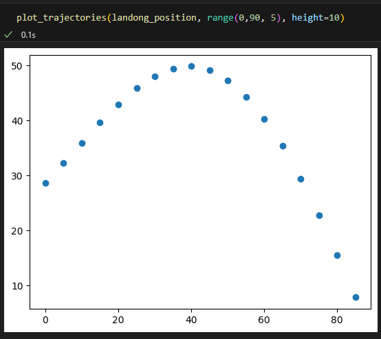
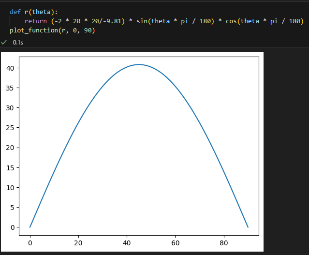
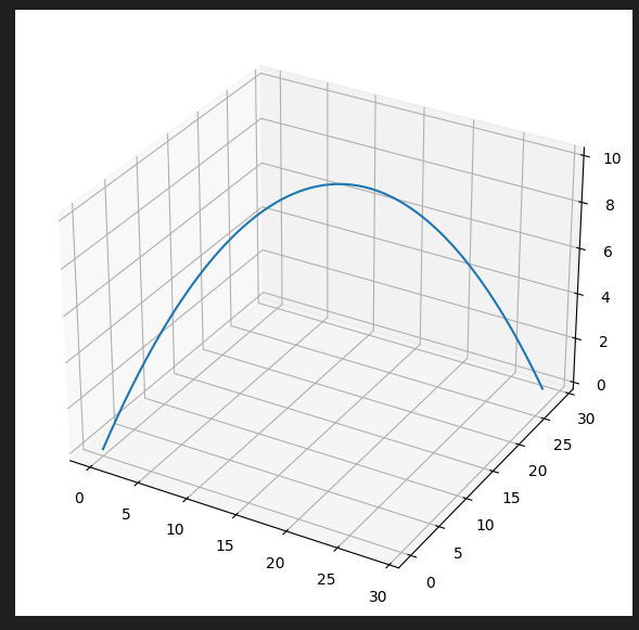
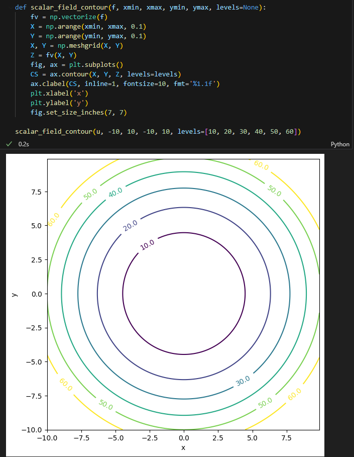
발사체의 최대거리 함수 r(theta)가 있을시, 거리를 최대로 하는 theta를 찾는 문제를 다룬다고 하자
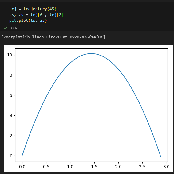
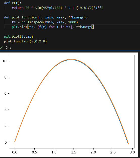
일단 발사체 궤적과 플로팅 함수는 다음과 같다
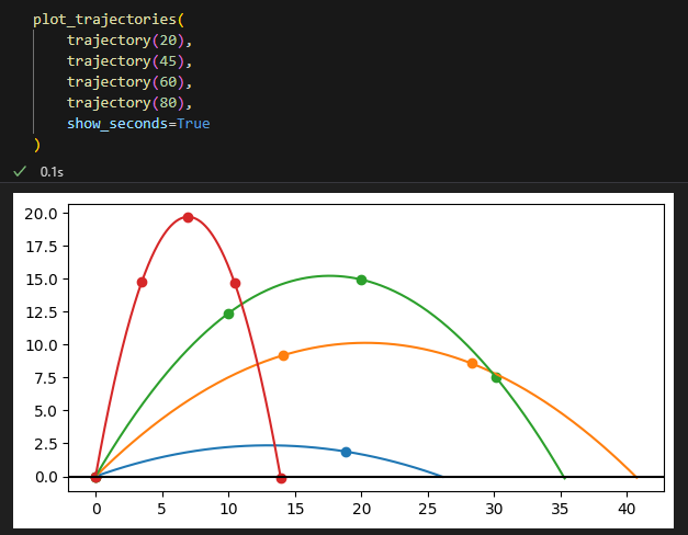
vx, vz는 속도를 xy축으로 분해한 성분으로
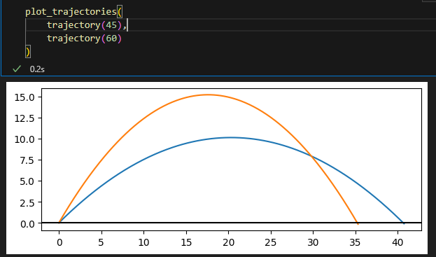
궤적 루프는 z가 0이 될때 즉 발사체가 땅으로 떨어지면 종료한다.
import matplotlib.pyplot as plt
from matplotlib import cm
import numpy as np
from math import sin, cos, pi

def trajectory(theta, speed=20, height=0, dt=0.01, g=-9.81):
    vx = speed * cos(pi * theta / 180)
    vz = speed * sin(pi * theta / 180)
    t, x, z = 0, 0, height
    ts, xs, zs = [t], [x], [z]
    while z >= 0:
        t += dt
        vz += g * dt
        x += vx * dt
        z += vz * dt
        ts.append(t)
        xs.append(x)
        zs.append(z)
    return ts, xs, zs

def plot_trajectories(*trajs, show_seconds=False):
    for traj in trajs:
        xs, zs = traj[1], traj[2]
        plt.plot(xs, zs)
        if show_seconds:
            second_indices = []
            second = 0
            for i, t in enumerate(traj[0]):
                if t >= second:
                    second_indices.append(i)
                    second +=1
            plt.scatter([xs[i] for i in second_indices], [zs[i] for i in second_indices])
    xl = plt.xlim()
    plt.plot(plt.xlim(), [0, 0], c='k')
    plt.xlim(*xl)

    width = 7
    coords_height = (plt.ylim()[1] - plt.ylim()[0])
    coords_width = (plt.xlim()[1] - plt.xlim()[0])
    plt.gcf().set_size_inches(width, width * coords_height / coords_width)
from vectors import to_polar, to_cartesian
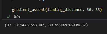
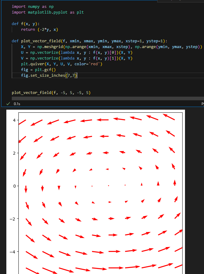
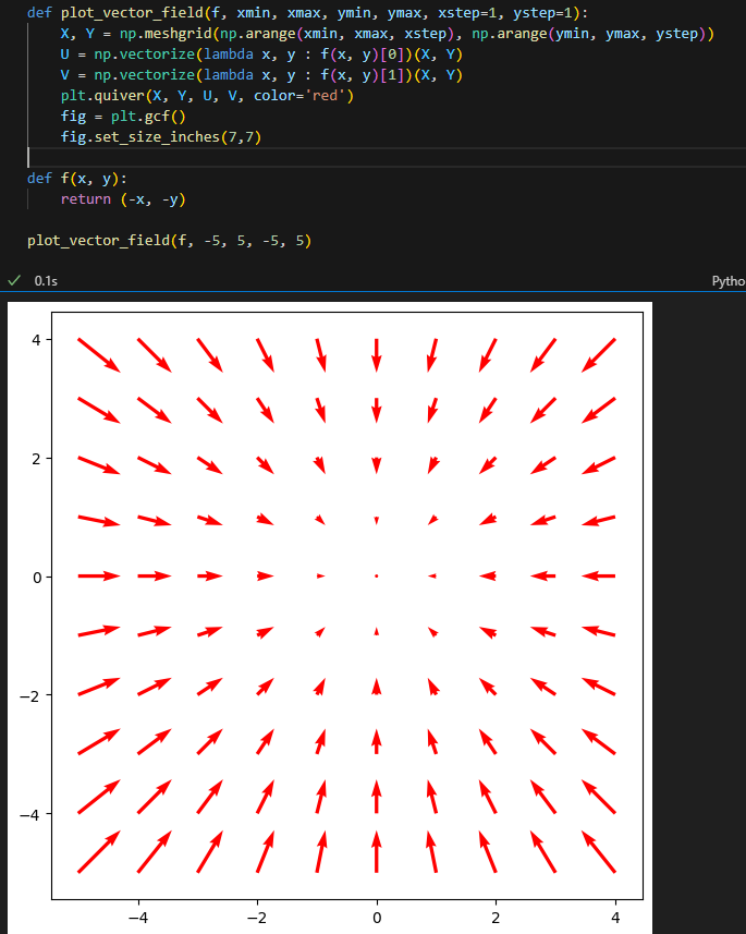
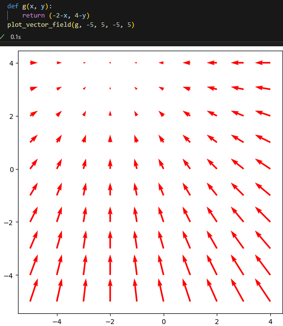
def plot_vector_field(f, xmin, xmax, ymin, ymax, xsteps=10, ysteps=10, color='k'):
X, Y = np.meshgrid(np.linspace(xmin,xmax,xsteps), np.linspace(ymin, ymax, ysteps))
U = np.vectorize(lambda x, y : f(x, y)[0])(X, Y)
V = np.vectorize(lambda x, y : f(x, y)[1])(X, Y)
plt.quiver(X, Y, U, V, color=color)
fig = plt.gcf()
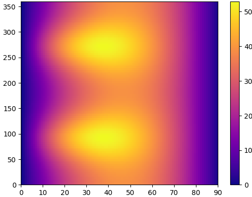
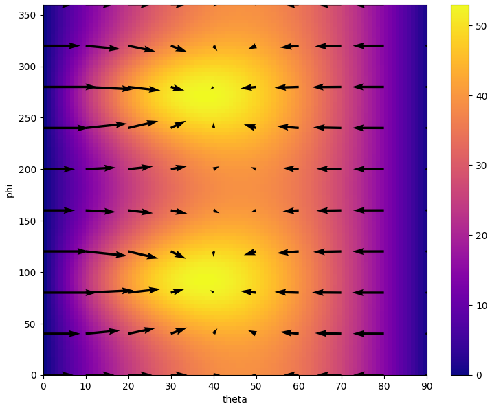
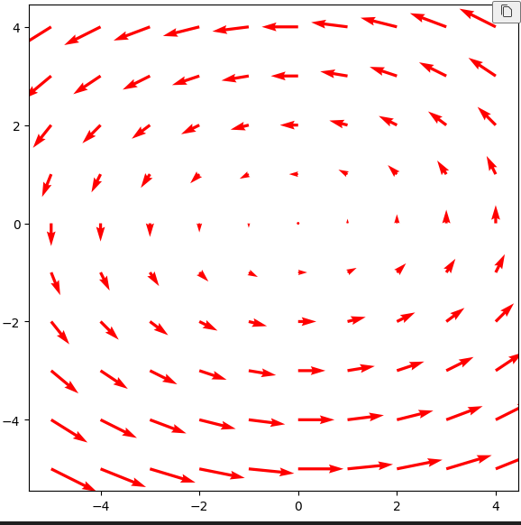
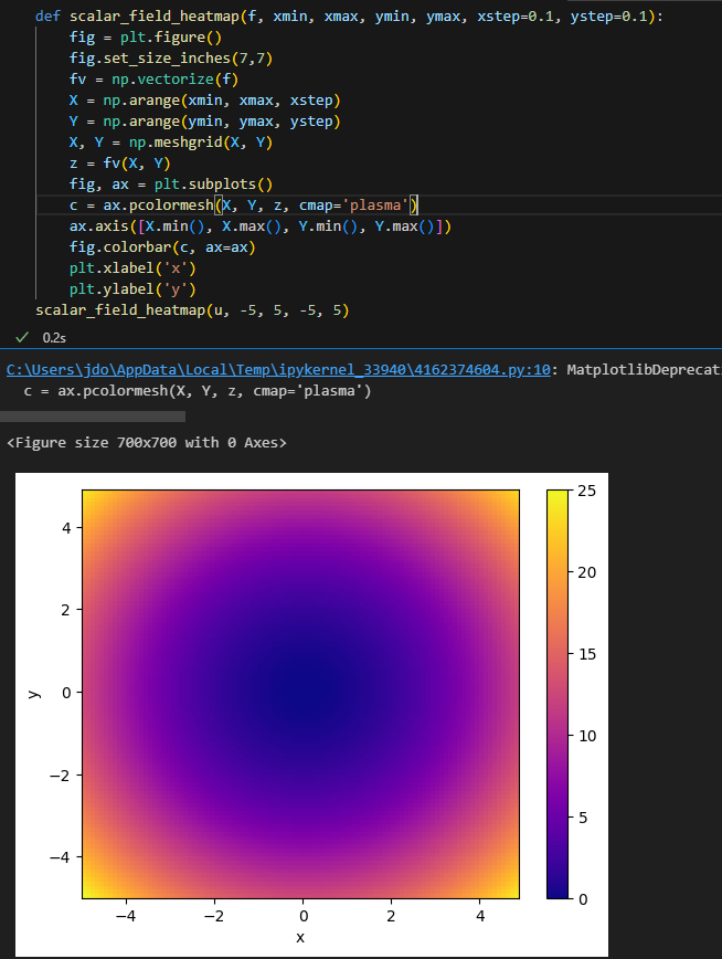
scalar_field_heatmap(landing_distance, 0, 90, 0, 360)
plot_vector_field(landing_distance_gradient, 0, 90, 0, 360, xsteps=10, ysteps=10, color='k')
plt.xlabel('theta')
plt.ylabel('phi')
plt.gcf().set_size_inches(9, 7)
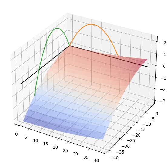
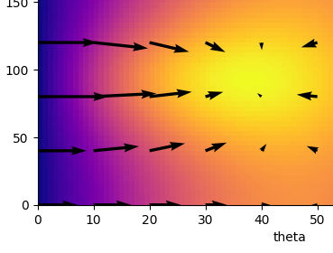
(2) 경사 상승법 구현하기
위에서 근사치 그라디언트 함수를 작성하여 벡터장 플로팅까지 했다
이번에는 이 근사 그라디언트로 경사 방향을 계속 올라 최대 지점까지 가는 함수 구현
36, 83을 줄시
끝점 37.58, 89.9에 도달함
from vectors import length

def gradient_ascent(f, xstart, ystart, tolerance=1e-6):
    x = xstart
    y = ystart
    grad = approx_gradient(f, x, y)
    while length(grad) > tolerance:
        x += grad[0]
        y += grad[1]
        grad = approx_gradient(f, x, y)
    return x, y

gradient_ascent(landing_distance, 36, 83)
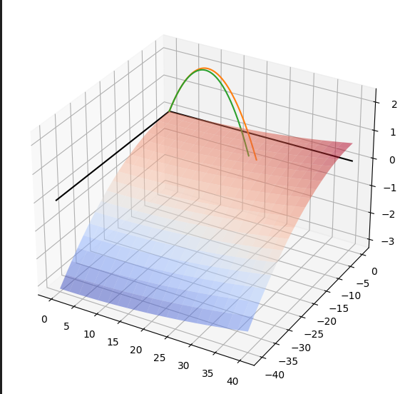
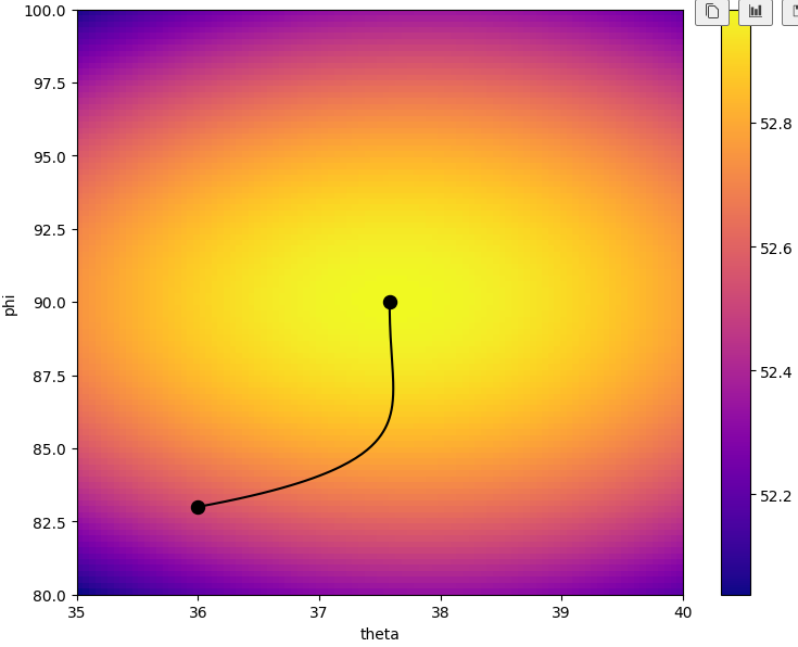
(3) 경사 상승 궤적 그리기
그라디언트 어센트 함수로 시작점을 주면 최적의 지점까지 찾는건 잘 됬는데
궤적을 드로잉해보면 다음과 같음
def gradient_ascent_points(f, xstart, ystart, tolerance=1e-6):
    x = xstart
    y = ystart
    xs, ys = [x], [y]
    grad = approx_gradient(f, x, y)
    while length(grad) > tolerance:
        x += grad[0]
        y += grad[1]
        grad = approx_gradient(f, x, y)
        xs.append(x)
        ys.append(y)
    return xs, ys

scalar_field_heatmap(landing_distance, 35, 40, 80, 100)

plt.plot(*gradient_ascent_points(landing_distance, 36, 83), c='k')
plt.scatter([36,37.58114751557887],[83,89.99992616039857],c='k',s=75)
plt.xlabel('theta')
plt.ylabel('phi')
plt.gcf().set_size_inches(9, 7)
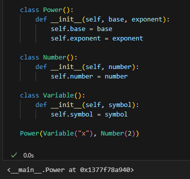
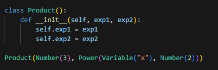
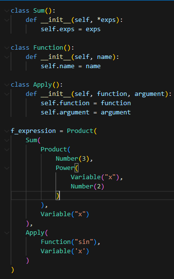
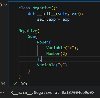
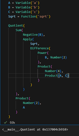
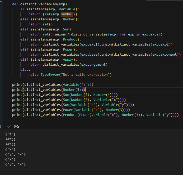
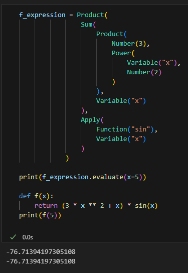
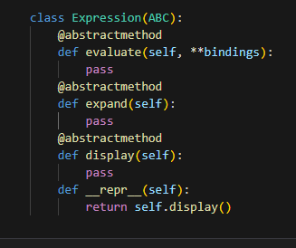
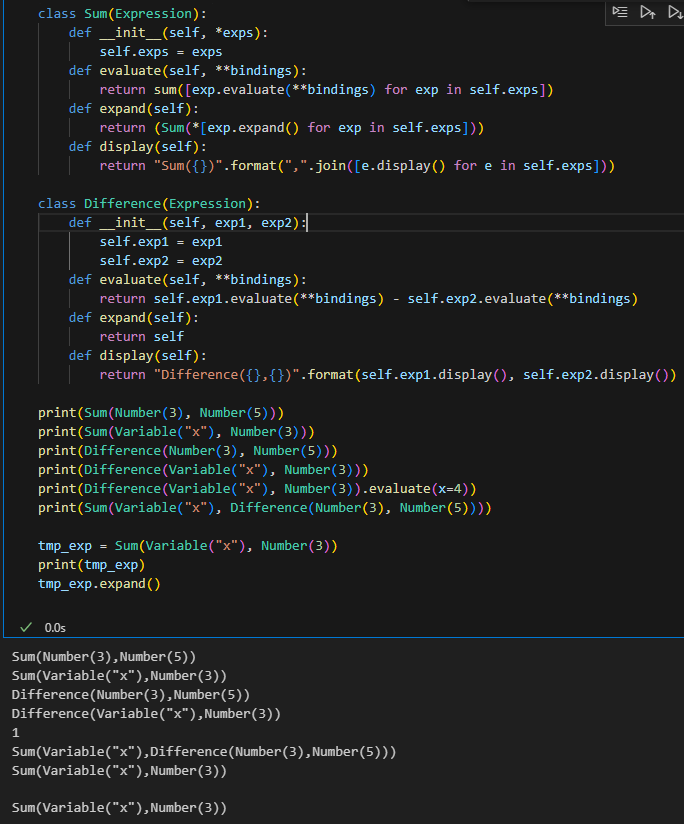
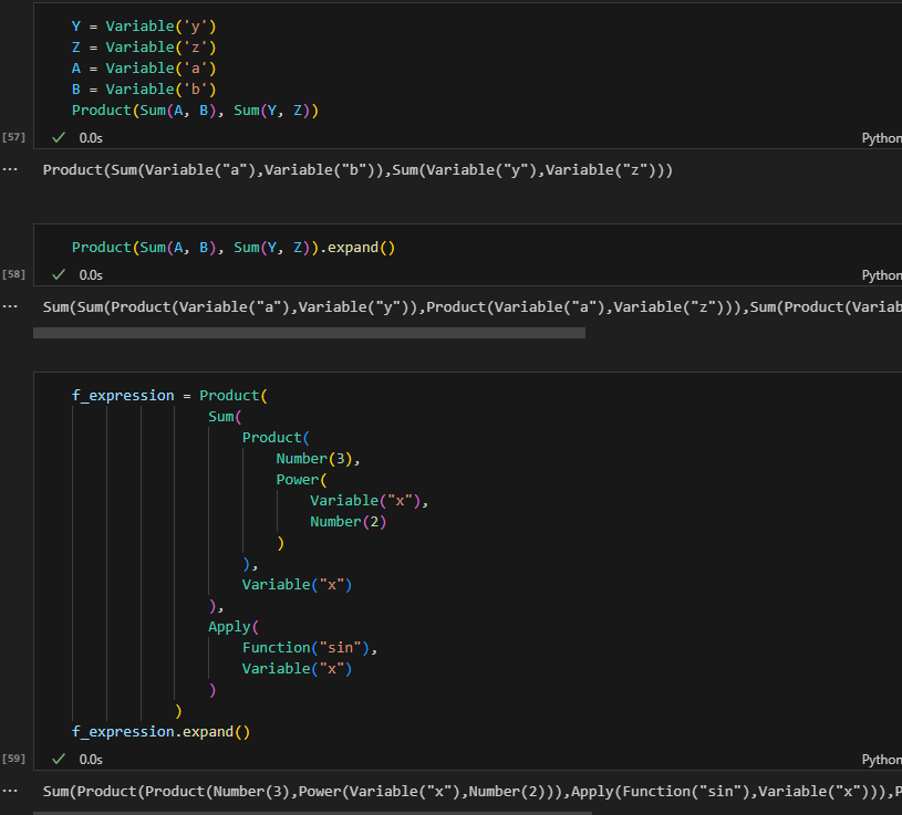
class Power():
def __init__(self, base, exponent):
self.base = base
self.exponent = exponent
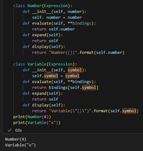
class Number():
def __init__(self, number):
self.number = number
class Variable():
def __init__(self, symbol):
self.symbol = symbol
Power(Variable("x"), Number(2))